Exercise #1
1.The gray level distribution of a 5X5, 3 bit image is shown as follows:
7 5 7 0 0
0 6 3 1 4
0 2 5 1 2
1 0 0 5 1
1 1 7 7 3
(1) Please plot the histogram, accumulated histogram, vertical and horizon
projection
histogram.
(2) Show the histogram after gray level sliding +2.
(3) Show the histogram after gray level extension 2.
(4) Show the gray level distribution after contrast enhancement between +3 and +5.
(5) Show the gray level distribution after low pass filter operation with the mask:
[ 1/9, 1/9, 1/9
1/9, 1/9, 1/9
1/9, 1/9, 1/9 ]
(6) Show the histogram after linearize.
2. A one-dimension signal x[n]=
[1 , 2 , 1, 3 , 5, 6, -1, -3, -5, -3, 1, 5, 6, 2, 1, 3, -1, 0, 2]
(1) Calculate the result of x[n] after a high pass operation (H(z)=1-0.95/z).
(2) Calculate the autocorrelation of x[n].
(3) Calculate x[n]*m[n], where m[n]=[ 1/3 , 1/3 , 1/3] .
(4) Calculate the crossing zero number of x[n].
1. A mask is shown as follows:
1/9 1/9 1/9
1/9 1/9 1/9
1/9 1/9 1/9
Please verify the high frequency will decay in this low pass filter operation.
2. A one-dimension signal x[n]=[1 , 2 , 1, 3 , 5, 6, -1, -3]
Please calculate the result X[k] of x[n] after FFT operation.
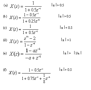
3. Determine the inverse z-transform:
4. A matlab program is written as follows:
t = 0:.001:1;
x = sin(2*pi*90*t) + sin(2*pi*1000*t);
y = x + 2*randn(size(t));
Y = fft(y);
Pyy = Y.*conj(Y);
plot(Pyy), title('Power spectral density'), ...
xlabel('Frequency'),
figure
t = 0:.001:2;
x = sin(2*pi*90*t) + sin(2*pi*1000*t);
y = x + 2*randn(size(t));
Y = fft(y);
Pyy = Y.*conj(Y);
plot(Pyy), title('Power spectral density'), ...
xlabel('Frequency'),
Please roughly plot the results of the spectrum.
Solution:
t = 0:.001:2;
x = sin(2*pi*90*t) + sin(2*pi*1000*t);
y = x + 2*randn(size(t));
Y = fft(y);
Pyy = Y.*conj(Y);
plot(Pyy), title('Power spectral density'), ...
xlabel('Frequency'),
pause
y=[1 , 2 , 1, 3 , 5, 6, -1, -3]
x=fft(y)
14.0000 -11.0711 - 3.4142i 6.0000 - 8.0000i 3.0711 + 0.5858i
-2.0000 3.0711 - 0.5858i 6.0000 + 8.0000i -11.0711 + 3.4142i


1. The gray level distribution of a 5X5, 3 bit image is shown as follows:
1 0 7 0 0
0 1 3 1 4
0 2 5 1 2
1 0 0 5 1
1 1 0 0 3
(1) Please plot the accumulated histogram.
(2) Show the histogram after gray level sliding -2.
(3) Show the gray level distribution after high pass filter operation with the mask:
[ -1, -1, -1
-1, 9 , -1
-1, -1, -1 ]
2. A one-dimension signal x[n]=
[1 , 5 , 2, -3 , -5, 0, 6, -1, -3, -5, -3, 1, 5, 6,-2, 1, 3, -1, 0, 2]
(1) Calculate the result of x[n] after a high pass operation (H(z)=1-0.9/z).
(2) Calculate x[n]*m[n], where m[n]=[ 1, 2, -1] .
(3) Calculate the crossing zero number of x[n].
3. Explain what is (a) Gibbs phenomenon (b) Nyquist frequency .
4. The sequence x[n]=cos(0.01 n) , -( < n < (
was obtained by sampling an analog signal xc[t]=cos(( t) , -( < t < (
at a sampling rate of 1 MHz. What are two possible values of ( that could
have resulted in the sequence x[n]?
5. Let h(t) denotes the impulse response of a linear time-invariant continuous-time
filter :
h(t)= exp(-3t) , when t ( 0
h(t)=0 , when t < 0
determine the continuous-time filter frequency response and sketch its magnitude.
6. Determine the z-transform, include the ROC, for the sequence:
0.3^n u [n]
1. A one-dimension signal x[n]=[-1 , -2 , 1, -3 ]
Please calculate the result X[k] of x[n] after FFT operation.
2. A discrete-time lowpass filter is to be designed by applying the impulse invariance method to a continuous-time Butterworth filter having magnitude-squared function
The specification for the discrete-time system are :
Sampling rate is 0.0001 samples/s
0.8 ( ( 1 , 0 ( (( 0.2 (
0( ( 0.1, 0.5 ((( ( (
Neglect the aliasing problem.
(a) Plot the tolerance scheme.
(b) Determine the integer order N and the quantity Td(c.
3. A matlab program:
wp=1000/10000;
ws=4000/10000;
[n,wn]=buttord(wp,ws,2,30)
[b,a]=butter(n,wn);
freqz(b,a,10000);
plot(abs(freqz(b,a,10000)))
please sketch the result:
4. Explanation:
(1) Band pass filter
(2) Butterworth lowpass filter
(3) isolated point
(4) chain code
Excercise #5
1. A one-dimension signal x[n]=[-1 , -2 , -1, 3 , 5, -6, -1,3]
Please calculate the result X[k] of x[n] after FFT operation.
2. A matlab program is written as follows:
t = 0:.01:30;
x = sin(2*pi*90*t) + sin(2*pi*400*t);
y = x + 2*randn(size(t));
Y = fft(y);
Pyy = Y.*conj(Y);
plot(Pyy), title('Power spectral density'), ...
xlabel('Frequency'),
Please roughly plot the results of the spectrum.
3. A binary image:
0 1 0 0 0 1 1 1
1 1 1 0 0 0 1 1
1 0 1 1 0 0 1 1
1 1 1 1 0 0 0 0
1 0 1 1 1 1 1 0
0 0 0 0 1 1 1 0
1 0 0 0 1 0 1 1
0 0 0 0 1 1 1 1
(1) Show the binary code distribution after open operation.
(2) Show the binary code distribution after close operation.
4. Explanation:
(1) Tustin transformation
(2) FIR filter
(3) Notch filter
(4) Butterworth lowpass filter
(5) isolated point
(6) chain code
5. A matlab program:
wp=1000/10000;
ws=4000/10000;
[n,wn]=buttord(wp,ws,1,15)
please calculate the result of n and wn:
Exercise #6
7 1 3 0 0
0 6 3 1 2
0 2 5 1 2
1 6 0 3 1
1 1 7 7 4
(1) Show the gray level distribution after 3(3 Median Filter operation.
(2) Show the binary code distribution, the background :0 and the object :1, after resholding operation ( thresholding value =4).
(3) The object in the binary image is a curve. Please show the pixel orientations
and chain code of this curve ( start at the left uppest point).
Sol:(1)
7 1 3 0 0
0 3 2 2 2
0 2 3 2 2
1 1 3 3 1
1 1 7 7 4
(2)
1 0 0 0 0
0 1 0 0 0
0 0 1 0 0
0 1 0 0 0
0 0 1 1 1
(3) pixel orientations: left uppest point 7 7 5700
chain code: left uppest point 111 111 101 111 000 000
2. A binary image:
0 1 0 0 0 1 0 0
1 1 1 0 0 0 0 0
1 0 1 1 0 0 1 0
1 1 1 1 0 0 0 0
1 0 1 1 1 1 1 0
0 0 0 0 1 1 1 0
1 0 0 0 1 0 1 1
0 0 0 0 1 1 1 1
(1) Show the binary code distribution after dilation operation.
(2) Show the binary code distribution after erosion operation.
(3) Show the binary code distribution after we compensate the missing point.
(4) Show the binary code distribution after we delete the isolated point.
Solution:(1)
1 1 1 1 1 1 1 0
1 1 1 1 1 1 1 1
1 1 1 1 1 1 1 1
1 1 1 1 1 1 1 1
1 1 1 1 1 1 1 1
1 1 1 1 1 1 1 1
1 1 0 1 1 1 1 1
1 1 0 1 1 1 1 1
(2)
0 0 0 0 0 0 0 0
0 0 0 0 0 0 0 0
0 0 0 0 0 0 0 0
0 0 0 0 0 0 0 0
0 0 0 0 0 0 0 0
0 0 0 0 0 0 0 0
0 0 0 0 0 0 0 0
0 0 0 0 0 0 0 0
(3)
0 1 0 0 0 1 0 0
1 1 1 0 0 0 0 0
1 1 1 1 0 0 1 0
1 1 1 1 0 0 0 0
1 0 1 1 1 1 1 0
0 0 0 0 1 1 1 0
1 0 0 0 1 1 1 1
0 0 0 0 1 1 1 1
(4)
0 1 0 0 0 0 0 0
1 1 1 0 0 0 0 0
1 0 1 1 0 0 0 0
1 1 1 1 0 0 0 0
1 0 1 1 1 1 1 0
0 0 0 0 1 1 1 0
0 0 0 0 1 0 1 1
0 0 0 0 1 1 1 1
3. Consider a stable linear time-invariant discrete-time system with input x[n] and
output y[n]. The input and output satisfy the difference equation
y[n-1]- (10/3) y[n] +y[n+1] =x[n]
(a) Plot the poles and zeros in the z-plane.
(b) Find the impulse response h[n].
4. Determine the system function of the two networks in Fig.6.1 and show that they
have the same poles.
5. A discrete-time lowpass filter is to be designed by applying the impulse invariance method to a continuous-time Butterworth filter having magnitude-squared function
The specification for the discrete-time system are :
Sampling rate is 0.0001 samples/s
0.89125< (|Hc|^2 < 1 ,
0<|Hc|^2< 0.17783,
Neglect the aliasing problem.
(a) Plot the tolerance scheme.
(b) Determine the imteger order N and the quantity Td.
5.A matlab program:
wp=2000/10000;
ws=3000/10000;
[n,wn]=buttord(wp,ws,1,15)
pause
[b,a]=butter(n,wn);
freqz(b,a,10000);
figure
plot(abs(freqz(b,a,10000)))
please sketch the result:
Ans:

Exercise #7
1. A mask is shown as follows:
1/9 1/9 1/9
1/9 1/9 1/9
1/9 1/9 1/9
Please verify the high frequency will decay in this low pass filter operation.
2. A one-dimension signal x[n]=[1 , 2 , 1, 3 , 5, 6, -1, -3]
Please calculate the result X[k] of x[n] after FFT operation.
3. Determine the inverse z-transform:

4. A matlab program is written as follows:
t = 0:.001:1;
x = sin(2*pi*90*t) + sin(2*pi*1000*t);
y = x + 2*randn(size(t));
Y = fft(y);
Pyy = Y.*conj(Y);
plot(Pyy), title('Power spectral density'), ...
xlabel('Frequency'),
figure
t = 0:.001:2;
x = sin(2*pi*90*t) + sin(2*pi*1000*t);
y = x + 2*randn(size(t));
Y = fft(y);
Pyy = Y.*conj(Y);
plot(Pyy), title('Power spectral density'), ...
xlabel('Frequency'),
Please roughly plot the results of the spectrum.